The long tail of El Nino
by JPMorgan
1 The long tail of El Niño: What to watch in 2027: Heat, commodity markets and mounting pressure on water
2 Executive Summary Many people are talking about El Niño, and I’ve been fielding a lot of questions from clients about what it means for economic impacts, planning and decision-making. We live in a world generally built for an average climate, with historic temporary swings we recover from but are not immune to. El Niño is a natural phenomenon where the ocean, acting like a heat battery, raises regional and global temperatures. However, with the climate changing in the background, this El Niño is already breaking records, with effects having started in late spring 2026 and continuing into 2027 and beyond across geographies and sectors. Some effects are already clear, with increased agriculture futures prices and land and ocean protein input costs. Others remain to be seen, including coral reef recovery as waters cool after the El Niño peak, potential drought in 2027 after the winter rainy season, and re-emergence (or not) of energy, industry and transportation disruptions caused by 2026’s hot summer drought. Temporary warming from El Niños can also serve as a useful planning tool, in that they provide a glimpse into what the status quo could be in a constantly hotter world. In an El Niño year, the temporary heat spike of a single month or season temporarily matches climate projections for average temperatures in coming years. Specifically in 2025, global temperatures were 1.3°C above pre-industrial levels i; in the future, scientists project annual average temperatures to exceed 1.5°C in the 2030s, 1.7°C in the 2040s, and 2.0°C in the 2050s. ii In the coming months, scientists predict winter temperatures about 1.7–1.8°C above pre-industrial levels and early-summer temperatures about 1.6°C above pre-industrial levels. In other words, this El Niño will show us what life may look like if these levels become our “new normal.” Climate models give us many timelines and worlds that offer theoretical views of temperature, precipitation, and storms, but must be translated into societal impacts. However, we only experience, or in scientific terms “observe,” one timeline and one world and its socioeconomic impact. An El Niño is a temporary extreme world: it heats the planet and shows us what is vulnerable and what is secure as climate conditions move beyond the accustomed ranges. A single year of extremes cannot tell us the full range or probability of future climate conditions, but it can act as a single observed stress test, potentially revealing where systems are vulnerable and where they prove more resilient. That can help identify the places and sectors where adaptation is most needed, and those that may be better positioned for the changes ahead. In this moment, we can learn from the temporary El Niño-induced spike in temperature and then prepare socially and economically for a hotter world. Impacts have historically been felt on ecosystems, geographies and real assets that are not resilient to climate variability. This is especially true for food production on land and sea, and countries with heavy dependencies on agriculture, fisheries and tourism. During an El Niño in a time of climate change, we may find that the additional temperature spike bringing record warm temperatures may also adversely impact real assets and industry built for cooler conditions: infrastructure, industrial coolant systems, energy production and buildings.
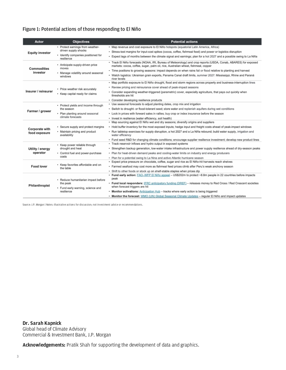
3 Dr. Sarah Kapnick Global head of Climate Advisory Commercial & Investment Bank, J.P. Morgan Acknowledgements: Pratik Shah for supporting the development of data and graphics. Source: J.P. Morgan | Notes: Illustrative actions for discussion; not investment advice or recommendations. Figure 1: Potential actions of those responding to El Niño
4 In May 2026, I published analysisiii on how fertilizer supply chain shocks and climate variability impact planting windows, crop yields and food inflation risk. Financial markets historically have responded the most to the first El Niño declaration (usually in June) vs. subsequent monthly forecasts.iv A prime time for equity markets to react has typically been before June (when the 2026 El Niño was first declared by the United States). However, agricultural productivity is the sum of crop inputs and the summation of many weather events over time (the climate of the growing season), which alters production outlooks and futures prices as decisions are made and new information comes in.
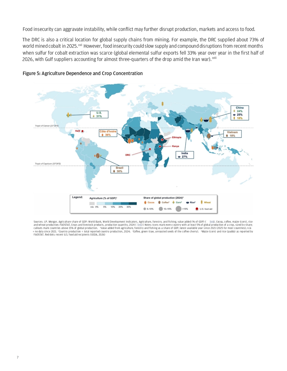
- Agriculture impacts 2026–2027 Figure 2: Commodity Futures Source: Bloomberg as of Nov. 2, 2026; futures curves (Bloomberg generic tickers) : CC1 Comdty NYB-ICE (cocoa), C 1 COMB Comdty CBT (corn), KC1 Comdty NYB-ICE (coffee), RR1 Comdty CBT (rough rice), W 1 COMB Comdty CBT (wheat), S 1 COMB Comdty CBT (soybeans), SB1 Comdty NYB-ICE (sugar #11) | Notes: prices are end-of-day closes. Each line is the futures curve (price by contract month) as of the date shown (Feb. 27, 2026, pre-conflict; June 11, 2026, the day El Niño was declared; Nov. 2, 2026, current) In May 2026, an El Niño was forming alongside a fuel and fertilizer supply shock. We predicted impacts on soft commodities, and they have materialized: since El Niño was declared on June 11, futures prices have risen especially for El Niño-sensitive crops such as cocoa (40%), rice (37%) and coffee (17%).v Sugar has also risen (25%). Grain futures, however, have pared most of their earlier gains: corn is up 2% and wheat is down 2%. Currently, specific equatorial (i.e., historically the most adversely affected tropical) geographies are factoring in a growing El Niño and are expecting lower yields (e.g., Australian winter wheat).vi The European Central Bank (ECB) has done analysis showing a strong El Niño can raise global food commodity prices by up to 9%, with the peak about 16 months after the event begins.vii Food inflation typically follows the El Niño peak, after several months of disruptive weather accumulating into a lower harvest. The ECB’s September 2026 projections have euro area food inflation peaking at 3.4% in the third quarter of 2027.viii For those concerned about emerging sovereign risks that could affect economies and trade, crop production forecasts may also predict famine and conflict. With the growing El Niño, fertilizer impacts from the Iran conflict and compounding effects of reduced transport, food security is forecasted to decline, especially in Africa where production is particularly sensitive in 2027.
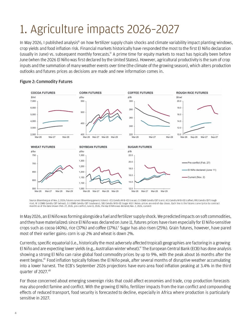
5 Figure 3: FEWS NET Food Security Outlook and History Source: FEWS NET, “2026-2027 El Niño food security impacts,” El Niño Special Report, Figure 2 and Table 1 (FEWS NET using USDA and NOAA data) ( link) | Notes: 1Timings to the nearest month; unimodal and bimodal = one and two main rainy seasons per year; food security bars include impacts from El Niño and other drivers; 2Each cell is the percent difference between production and normal production in the crop year of the event. Normal production is the level a crop’s long-run growth trend predicts for that year, estimated from up to seven years before and after it, with the strong and very strong El Niño years left out. Measuring against it keeps a crop’s steady growth from hiding a shortfall. 1986/87 and 1987/88 are the two crop years of one event (1986–1988). The average is taken per event across the seven events, with 1986–1988 counted as the mean of its two crop years Most major wheat exporters expect smaller 2026/27 harvests (USDA projects declines of 23% in the U.S., 10% in Australia and Canada, and 8% in the EU). Ukraine is the exception, with expected output up 10% to 26.5 million tons; Russia’s expected harvest dips 3% to 88.0 million tons, but its stocks are rebuilding (12.0 to 20.1 million tons).ix Historically, colder regions produce more grain during warmer El Niño temperatures, offsetting global supply losses from the equator.x However, the Russia–Ukraine conflict could inhibit the movement of grain out of Ukraine, with recent drone bombings of grain storage and disruption to ships leaving the region.xi This is something to watch; Ukraine’s larger harvest and Russia’s rebuilding stocks — the two countries together accounted for approximately 13.2% of global wheat production in 2024 — may not fully translate into additional supplies reaching global markets if conflict disrupts exports. xii
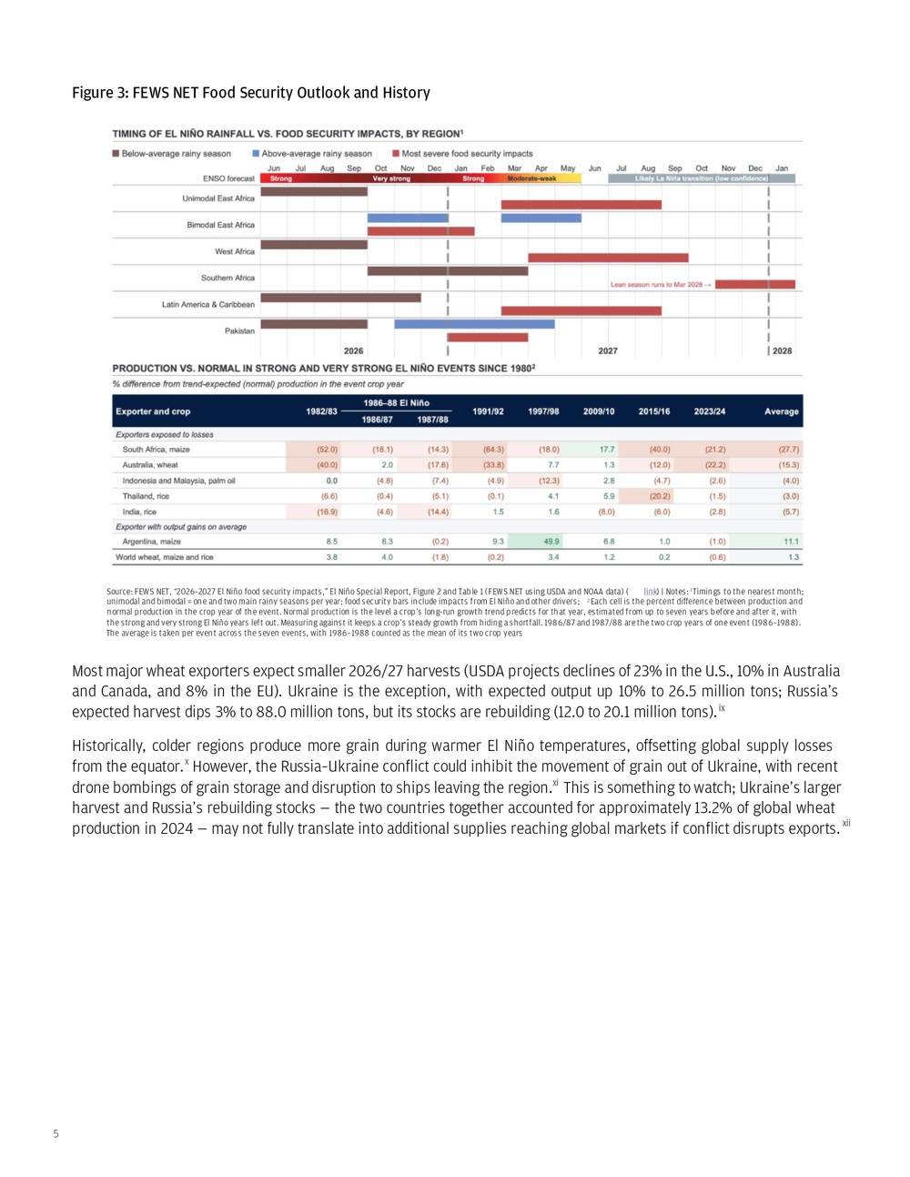
6 Figure 4: USDA Wheat Outlook Source: USDA Foreign Agricultural Service, Production, Supply and Distribution (PSD), November 2026 download ( link); November WASDE (link) | Notes: Marketing years; 2025/26 = USDA estimate; 2026/27F = USDA projection. Utilization = total domestic use (food, feed, seed and industrial); exports = trade-year (July–June) exports; closing stocks = end-of-year stocks While oil shipments have improved since the start of the Iran conflict, maritime transport has not fully normalized in the Strait of Hormuz or Red Sea, with container shipping costs up 131% since before the conflict.xiii Put together, production of staple crops is expected to be down in most places. The one place producing more is in active conflict (Ukraine), and pricing for fuel, shipping and fertilizer has been elevated throughout critical growing season points. Another important note: current supply-reduction forecasts are helping to elevate crop futures. These may drive consumer inflation through 2027, and, unlike other sources of inflation, are stickier because demand for staple foods is inelastic. Soft commodities are experiencing both supply and input inflationary price pressures in 2026. These pressures are expected to continue to affect crops harvested into 2027 as El Niño weather patterns peak by February, but the added heat from the ocean into the atmosphere is expected to keep global temperatures elevated through summer. Productivity forecasts do not currently cite exceptional, unprecedented summer 2027 heatwaves as a concern, but this may change in spring as the summer outlook becomes clearer. The U.S. government has recently restarted food aid after closing USAID in 2025, announcing $825 million in “America First” international food assistance (USDA), with the Food for Peace emergency share going to Ethiopia, Kenya, the Democratic Republic of the Congo and Haiti. This is on top of up to $452 million via World Food Programme (WFP) announced in February 2026 that includes the DRC, which maps onto the FAO food security concern locations.xiv These hotspots for food insecurity may also carry regional security implications: in eastern Africa, external trade shocks may compound existing conflict, climate stressxv and import dependence. The region is still grappling with the effects of severe drought, including five consecutive below-average rainy seasons in southern and southeastern Ethiopia through late 2022. In Kenya, drought has damaged maize and wheat harvests in parts of the country, disrupted rice cultivation through water rationing, and reduced livestock herds and milk production.xvi Here, higher fuel prices have also triggered a nationwide public transport strike and protests, illustrating how economic pressures can spill into public discontent.
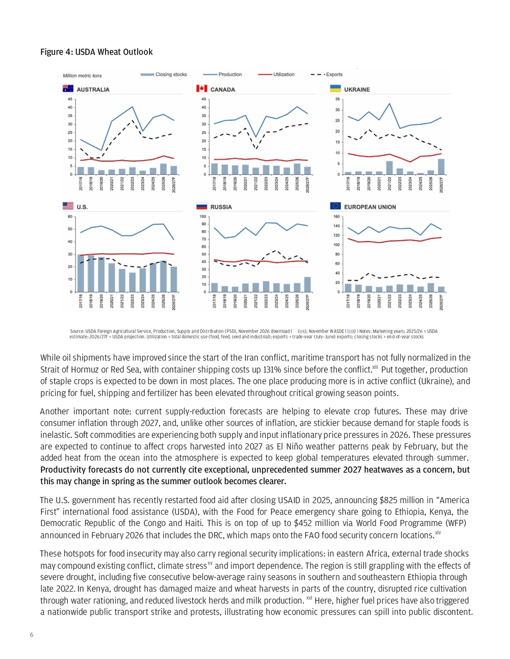
7 Figure 5: Agriculture Dependence and Crop Concentration Sources: J.P. Morgan. Agriculture share of GDP: World Bank, World Development Indicators, Agriculture, forestry, and fishing, value added (% of GDP) ( link). Cocoa, coffee, maize (corn), rice and wheat production: FAOSTAT, Crops and livestock products, production quantity, 2024 ( link) | Notes: Icons mark every country with at least 5% of global production of a crop, sized by share; callouts mark countries above 15% of global production. 1Value added from agriculture, forestry and fishing as a share of GDP; latest available year since 2021 (2025 for most countries); n/a = no data since 2021. 2Country production ÷ total reported country production, 2024; 3Coffee, green (raw, unroasted seeds of the coffee cherry). 4Maize (corn) and rice (paddy) as reported by FAOSTAT. Red dots: recent U.S. food aid recipients (USDA, 2026) Food insecurity can aggravate instability, while conflict may further disrupt production, markets and access to food. The DRC is also a critical location for global supply chains from mining. For example, the DRC supplied about 73% of world mined cobalt in 2025.xvii However, food insecurity could slow supply and compound disruptions from recent months when sulfur for cobalt extraction was scarce (global elemental sulfur exports fell 33% year over year in the first half of 2026, with Gulf suppliers accounting for almost three-quarters of the drop amid the Iran war).xviii
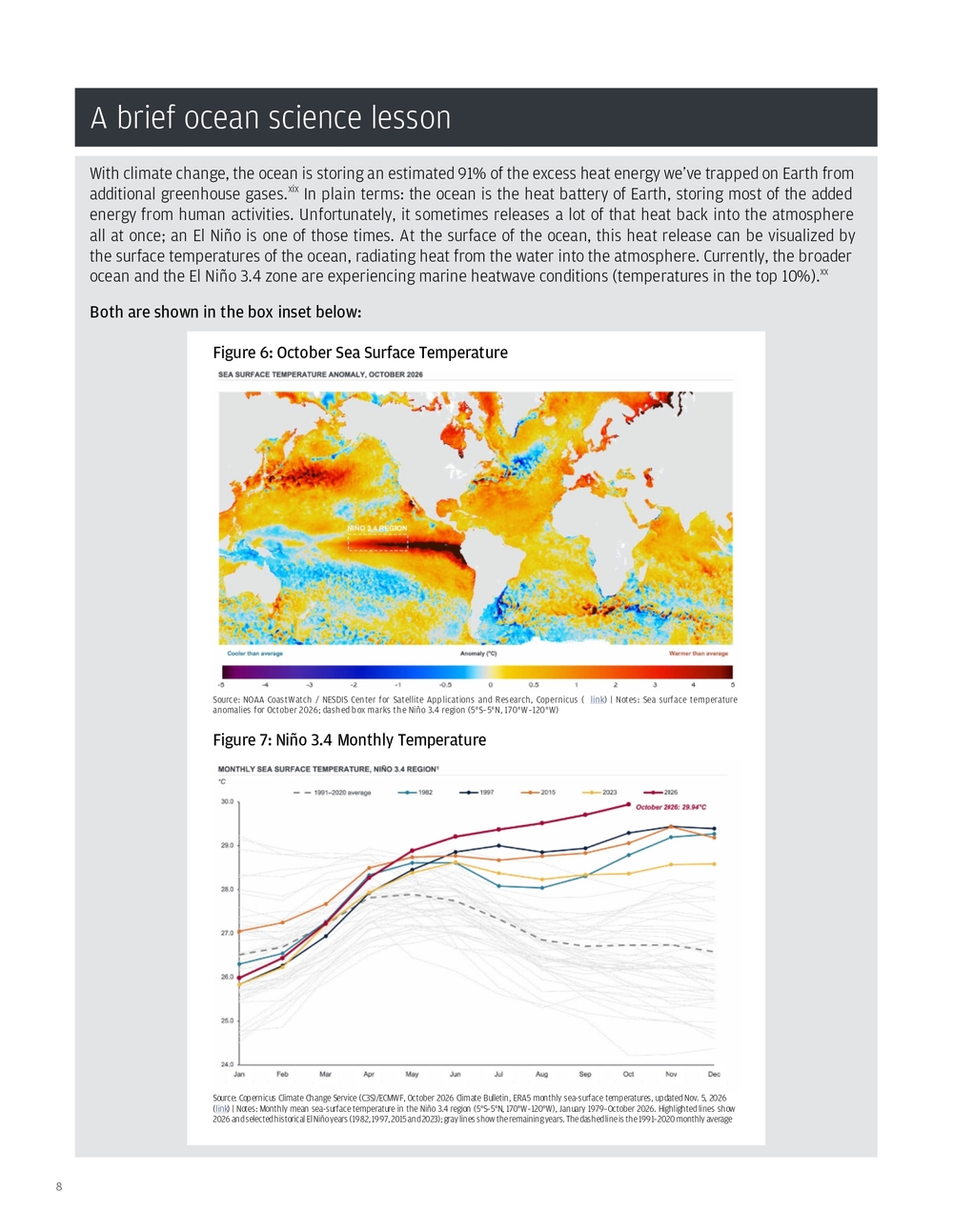
8 With climate change, the ocean is storing an estimated 91% of the excess heat energy we’ve trapped on Earth from additional greenhouse gases.xix In plain terms: the ocean is the heat battery of Earth, storing most of the added energy from human activities. Unfortunately, it sometimes releases a lot of that heat back into the atmosphere all at once; an El Niño is one of those times. At the surface of the ocean, this heat release can be visualized by the surface temperatures of the ocean, radiating heat from the water into the atmosphere. Currently, the broader ocean and the El Niño 3.4 zone are experiencing marine heatwave conditions (temperatures in the top 10%).xx Both are shown in the box inset below: A brief ocean science lesson Source: NOAA CoastWatch / NESDIS Center for Satellite Applications and Research, Copernicus ( link) | Notes: Sea surface temperature anomalies for October 2026; dashed box marks the Niño 3.4 region (5°S–5°N, 170°W–120°W) Figure 6: October Sea Surface Temperature Source: Copernicus Climate Change Service (C3S)/ECMWF, October 2026 Climate Bulletin, ERA5 monthly sea-surface temperatures, updated Nov. 5, 2026 (link) | Notes: Monthly mean sea-surface temperature in the Niño 3.4 region (5°S–5°N, 170°W–120°W), January 1979–October 2026. Highlighted lines show 2026 and selected historical El Niño years (1982, 1997, 2015 and 2023); gray lines show the remaining years. The dashed line is the 1991–2020 monthly average Figure 7: Niño 3.4 Monthly Temperature
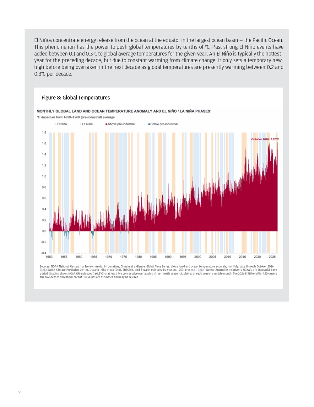
9 El Niños concentrate energy release from the ocean at the equator in the largest ocean basin — the Pacific Ocean. This phenomenon has the power to push global temperatures by tenths of °C. Past strong El Niño events have added between 0.1 and 0.3°C to global average temperatures for the given year. An El Niño is typically the hottest year for the preceding decade, but due to constant warming from climate change, it only sets a temporary new high before being overtaken in the next decade as global temperatures are presently warming between 0.2 and 0.3°C per decade. Figure 8: Global Temperatures Sources: NOAA National Centers for Environmental Information, Climate at a Glance: Global Time Series, global land and ocean temperature anomaly, monthly, data through October 2026 (link); NOAA Climate Prediction Center, Oceanic Niño Index (ONI), ERSSTv6, cold & warm episodes by season, 1950–present ( link) | Notes: 1Anomalies relative to NOAA’s pre-industrial base period. Shading shows NOAA ONI episodes ( ±0.5°C for at least five consecutive overlapping three-month seasons), plotted at each season’s middle month. The 2026 El Niño (MAM–ASO) meets the five-season threshold; recent ONI values are estimates and may be revised
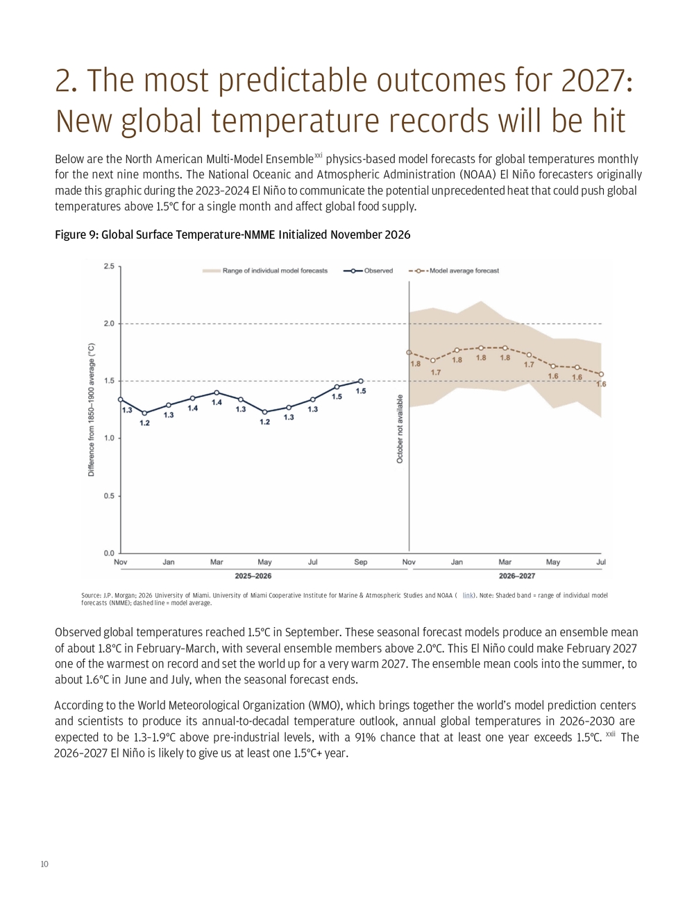
10 Below are the North American Multi-Model Ensemblexxi physics-based model forecasts for global temperatures monthly for the next nine months. The National Oceanic and Atmospheric Administration (NOAA) El Niño forecasters originally made this graphic during the 2023–2024 El Niño to communicate the potential unprecedented heat that could push global temperatures above 1.5°C for a single month and affect global food supply. 2. The most predictable outcomes for 2027: New global temperature records will be hit Figure 9: Global Surface Temperature-NMME Initialized November 2026 Source: J.P. Morgan; 2026 University of Miami. University of Miami Cooperative Institute for Marine & Atmospheric Studies and NOAA ( link). Note: Shaded band = range of individual model forecasts (NMME); dashed line = model average. Observed global temperatures reached 1.5°C in September. These seasonal forecast models produce an ensemble mean of about 1.8°C in February–March, with several ensemble members above 2.0°C. This El Niño could make February 2027 one of the warmest on record and set the world up for a very warm 2027. The ensemble mean cools into the summer, to about 1.6°C in June and July, when the seasonal forecast ends. According to the World Meteorological Organization (WMO), which brings together the world’s model prediction centers and scientists to produce its annual-to-decadal temperature outlook, annual global temperatures in 2026–2030 are expected to be 1.3–1.9°C above pre-industrial levels, with a 91% chance that at least one year exceeds 1.5°C. xxii The 2026–2027 El Niño is likely to give us at least one 1.5°C+ year.
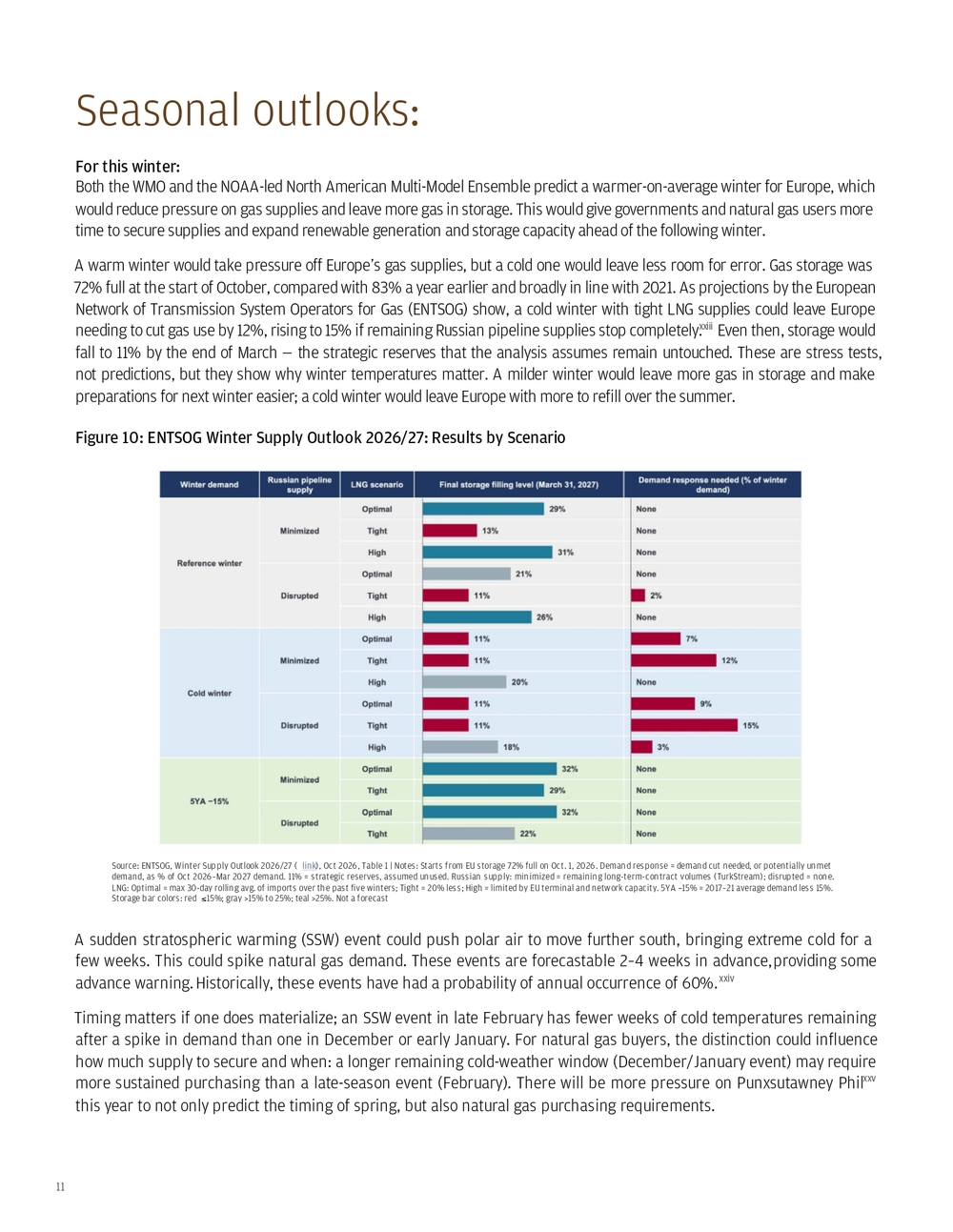
11 For this winter: Both the WMO and the NOAA-led North American Multi-Model Ensemble predict a warmer-on-average winter for Europe, which would reduce pressure on gas supplies and leave more gas in storage. This would give governments and natural gas users more time to secure supplies and expand renewable generation and storage capacity ahead of the following winter. A warm winter would take pressure off Europe’s gas supplies, but a cold one would leave less room for error. Gas storage was 72% full at the start of October, compared with 83% a year earlier and broadly in line with 2021. As projections by the European Network of Transmission System Operators for Gas (ENTSOG) show, a cold winter with tight LNG supplies could leave Europe needing to cut gas use by 12%, rising to 15% if remaining Russian pipeline supplies stop completely.xxiii Even then, storage would fall to 11% by the end of March — the strategic reserves that the analysis assumes remain untouched. These are stress tests, not predictions, but they show why winter temperatures matter. A milder winter would leave more gas in storage and make preparations for next winter easier; a cold winter would leave Europe with more to refill over the summer. A sudden stratospheric warming (SSW) event could push polar air to move further south, bringing extreme cold for a few weeks. This could spike natural gas demand. These events are forecastable 2–4 weeks in advance, providing some advance warning. Historically, these events have had a probability of annual occurrence of 60%.xxiv Timing matters if one does materialize; an SSW event in late February has fewer weeks of cold temperatures remaining after a spike in demand than one in December or early January. For natural gas buyers, the distinction could influence how much supply to secure and when: a longer remaining cold-weather window (December/January event) may require more sustained purchasing than a late-season event (February). There will be more pressure on Punxsutawney Phil xxv this year to not only predict the timing of spring, but also natural gas purchasing requirements. Seasonal outlooks: Figure 10: ENTSOG Winter Supply Outlook 2026/27: Results by Scenario Source: ENTSOG, Winter Supply Outlook 2026/27 ( link), Oct 2026, Table 1 | Notes: Starts from EU storage 72% full on Oct. 1, 2026. Demand response = demand cut needed, or potentially unmet demand, as % of Oct 2026–Mar 2027 demand. 11% = strategic reserves, assumed unused. Russian supply: minimized = remaining long-term-contract volumes (TurkStream); disrupted = none. LNG: Optimal = max 30-day rolling avg. of imports over the past five winters; Tight = 20% less; High = limited by EU terminal and network capacity. 5YA −15% = 2017–21 average demand less 15%. Storage bar colors: red ≤ 15%; gray >15% to 25%; teal >25%. Not a forecast
12 The El Niño and global temperature predictions also provide a forecast for real assets and labor resilience preparation for the summer of 2027. After record-breaking heatwaves rolled through much of the Northern Hemisphere in the summer of 2026, the need to adapt to build resilience to heat has been a topic of discussion. Extreme heat impacting infrastructure went from theoretical to real (e.g., rails and bridges buckling and shutting down transportation; heatstroke in outdoor workers and commuters on non-air-conditioned buses and rails across Europe; the melting of plastic casings, roads and tarmacs). We saw record heatwaves in a summer of observed global monthly temperatures of 1.3–1.5°C above pre-industrial levels (June–August 2026, University of Miami).xxvi The ensemble average forecast for global temperature is about 1.6°C above pre-industrial levels in June 2027. This could tip the likelihood for local heat extremes higher, with the potential for even more severe heatwaves in a warmer world. Summer of 2027:
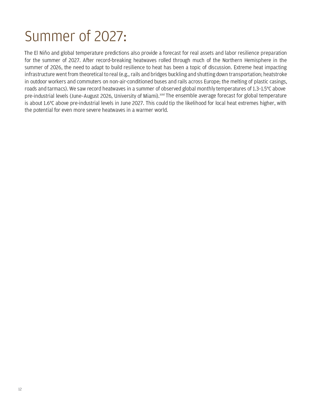
13 For this winter: Natural gas users and governments should have emergency response plans ready for how they will encourage demand reduction if an SSW event develops. Playbooks and engagement campaigns are best prepared in advance versus when an event is unfolding. A sudden stratospheric warming event in January will have more impact than one later in the season in February, as there are more weeks of winter to ensure supply security and potentially suppress demand. For summer 2027 and beyond: Treat the recent heatwaves as a test for the floor, not the ceiling, for temperatures in future years.xxvii And with next year baking in global temperatures with a baseline above those ever recorded, the winter respite from the just-recorded heatwaves should be used to identify failure points and critical areas for investment as even hotter heatwaves are likely next summer. A shift into a 2027-2028 La Nina could bring an active Atlantic hurricane season with La Nina reduced wind shear and still-elevated Atlantic Ocean temperatures Specific heat wave resilience plans: • Build out HVAC systems with battery storage to handle surges in energy consumption for residential and commercial properties. Heat pumps can provide summer cooling AND electrify winter heating to remove fossil fuel dependencies. But they will increase demand on the grid, requiring utilities to manage demand growth and potentially expand supply. • Upgrade efficient cooling systems for industry to ensure they can run during heatwaves, especially closed-loop systems if cold water is drawn from surface waters that are warming or becoming scarcer with increased air temperatures. • Create emergency and response plans, so you are ready to act when weather forecasts (two to four weeks ahead) are released. Then you can implement them as predefined thresholds are crossed to minimize workforce impacts, infrastructure damage, business interruptions or other losses. • Remember that even if your factory or office site has air conditioning and contingency plans, your workforce may not be able to get to it if public transportation or schools/childcare facilities shut down in a heatwave. My El Niño preparedness advice: Figure 11: El Nino Preparedness: What to Do and When Source: J.P. Morgan. Note: SSW = sudden stratospheric warming, a rapid warming of the polar stratosphere that can bring prolonged cold spells in the weeks that follow
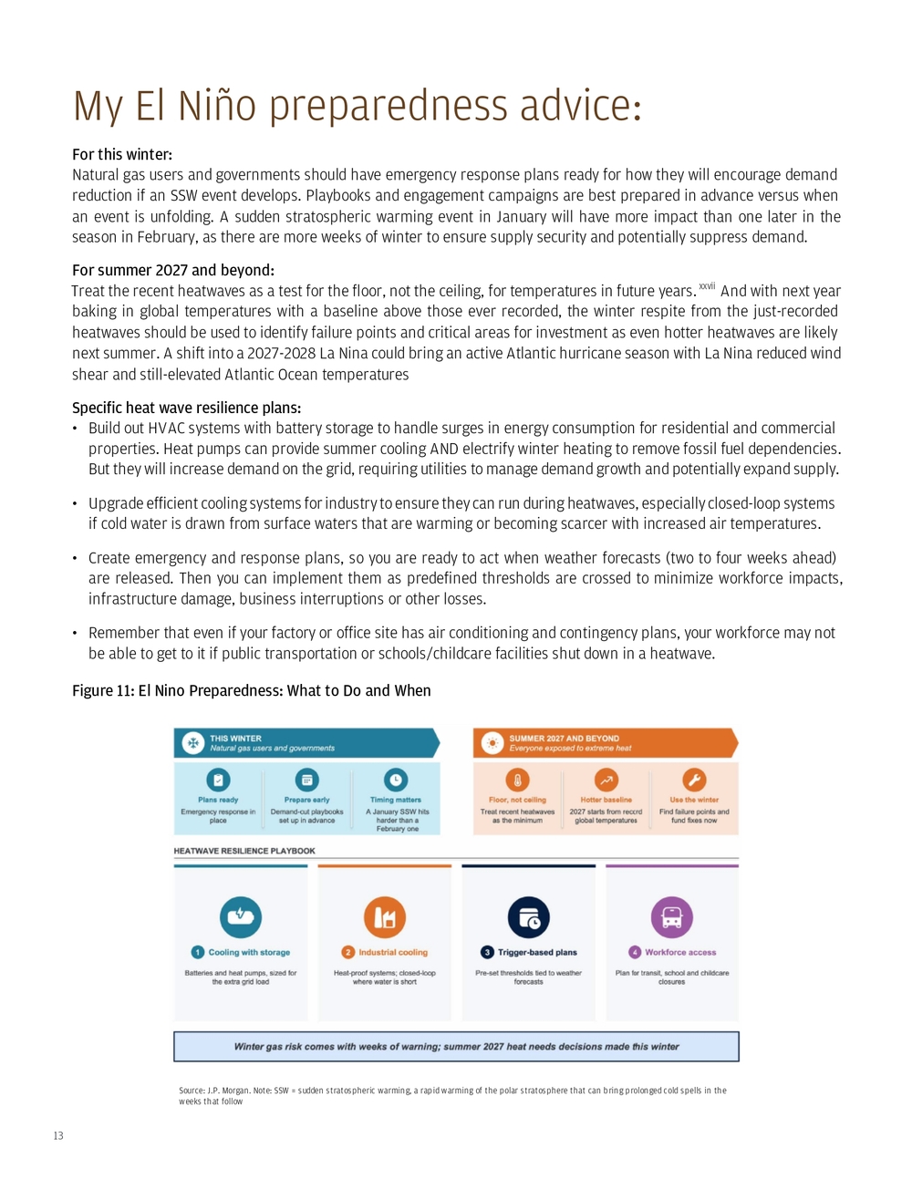
14 El Niño monitoring and climate prediction originally developed from a desire to predict ocean fisheries catch and agriculture output, after an unpredicted El Niño in 1972–1973 collapsed the anchovy fishery (largest commercial fishery at the time) off the coast of Peru. xxviii This motivated efforts to build statistical and later physical models of ocean observations to predict El Niños before they happen. In recent decades, this capability has developed, with buoys, undersea drone-like robotsxxix and satellite data providing information to feed into models based on physics, statistics, and increasingly AI. These are used to predict El Niños and their impacts, especially on fish, coral reefs and agriculture. El Niños in a time of climate change have short- and long-term impacts. In the short term: As historically strong El Niños have developed in spring, normally concentrated fish populations along the equator off the coast of South America disperse, seeking cooler food-rich waters elsewhere. This has historically collapsed the anchovy fishery off the coast of Peru. This happened in May and June 2026, with the anchovy fishery closing as fish became scarce, lowering GDP growth. xxx The shift from concentrated to dispersed fish made it hard to make up for their loss, and they reproduced at lower levels, seeking food elsewhere. The loss of fish catches immediately had a few impacts:
- Peru’s economy grew 1.8% year over year in May, below market expectations of 3.2% growth.xxxi
- It sent fishmeal prices, which depend on ocean-caught fish from this region, up 61% year over year by October 2026.
- Medium predictable: Coral reefs, fisheries and sovereign debt risk Figure 12: Fishmeal Prices Ease From September’s Record Sources: 1World Bank, Commodity Price Data (The Pink Sheet), monthly prices, fish meal (US$/mt), updated Nov. 3, 2026 ( link); 2FAO. 2024. The State of World Fisheries and Aquaculture 2024 – Blue Transformation in action. Rome. ( link) | Notes: Index January 2020 = 100. World Bank fish meal series: German 64% protein, EXW Hamburg, to Dec 2020; Danish 64% protein, FOB Bremen, Jan 2021–Jun 2026; herring fish meal 64% protein, FOB North Germany, from Jul 2026. End-market shares may not sum to 100% due to rounding
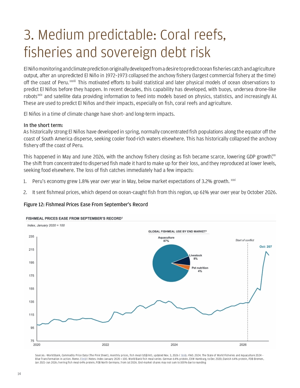
15 This fishery recovers almost immediately after temperatures return to normal, bringing cold, nutrient-rich water back to the equator. Until temperatures return to normal, fishmeal prices may remain elevated, potentially through spring 2027, increasing feed costs for aquaculture and livestock. In the long term: Since 1997, El Niño events amid a changing climate have subjected coral reefs to heat stress that can cause bleaching.xxxii If waters don’t cool within a few weeks or months, the corals bleach permanently and die. In the last global bleaching event (2023–2025), 84% of the world’s coral reef area experienced bleaching-level heat stress, and some species became functionally extinct in the Caribbean (i.e., there have been no more signs of reanimation or new growth of some coral species). It remains to be seen how much bleaching the current El Niño will cause and how widespread it will be. Figure 13: Changes in Hard Coral Cover at the Global Scale from 1980 to 2024 Sources: Status of Coral Reefs of the World: 2025. González-Rivero, M., Dallison, T., Wicquart, J., Brigdale, A., Logan, M., Fobert, E. K., Staub, F., and Planes, S. (eds.), 2026. Status of Coral Reefs of the World: 2025. Global Coral Reef Monitoring Network (GCRMN), International Coral Reef Initiative (ICRI). https://doi.org/10.59387/LFPR6347 ( link); ICRI/GCRMN, share of the world’s reefs under bleaching-level heat stress in each global bleaching event (2023–25 event to March 30, 2025) ( link)
16 On a broader scale, coral reefs support tourism, serve as nurseries for regional fish and absorb waves moving to shore, lowering erosion rates. Weakening coral reefs can lower tourism revenues, impact certain fish catches, and increase erosion rates, damaging coastal property. The most vulnerable coral reef countries to losses of fish and tourism are mapped below (see the figure notes for how each measure is calculated), along with their sovereign debt over GDP levels. Figure 14: Coral Stress and Economic Dependencies Sources: J.P. Morgan. Coral reef conditions: NOAA Coral Reef Watch, NOAA Coral Reef 5km Satellite Coral Bleaching Heat Stress Products (Version 3.1) – College Park, Maryland, U.S.: NOAA Coral Reef Watch ( link). Fisheries GDP: FAO GLOBEFISH ( link). Impacts of El Niño may suppress figures in regions near the equatorial Pacific. Fisheries figures cover only primary fisheries and aquaculture, excluding processing, trade and other revenue streams that cannot be consistently tracked globally under existing industrial classifications. Inbound tourism spending: UN Tourism inbound expenditure, total, latest year 2019–2024 ( link), © UN Tourism 2025, ÷ World Bank GDP (current US$), same year. Debt-to-GDP: IMF, World Economic Outlook (October 2026) ( link) | Notes: Selection of countries with fisheries around 1% of GDP or more in or near the coral heat-stress area shown, plus Peru (anchoveta fishery). *Vietnam spending 2019 (pre-COVID). Fisheries: 2024 for Vietnam, Philippines, Peru, Tuvalu; others 2023. Debt figures are for 2025. 1NOAA Coral Reef Watch Bleaching Alert Area Monthly Composites, Maximum Oct 2026; scale: No stress (clear), Watch, Warning, Alert Levels 1–5; clear = no data Unless these economies diversify, they have near- and longer-term exposure to coral reef bleaching and decline. The fisheries figures above understate the sector’s broader economic importance: they cover only primary fisheries and aquaculture production, excluding processing, trade and other revenue streams that cannot be consistently tracked globally under existing industrial classifications. The lack of standardized blue-economy metrics limits cross-country comparisons of the sector’s full economic contribution; these figures should therefore be viewed as a floor rather than a comprehensive measure. These omissions are particularly significant for processing hubs such as Seychelles and Vietnam. In Kiribati, for example, license fees from foreign fishing vessels — excluded from these figures — are thought to be equivalent to around 50% of GDP.xxxiii
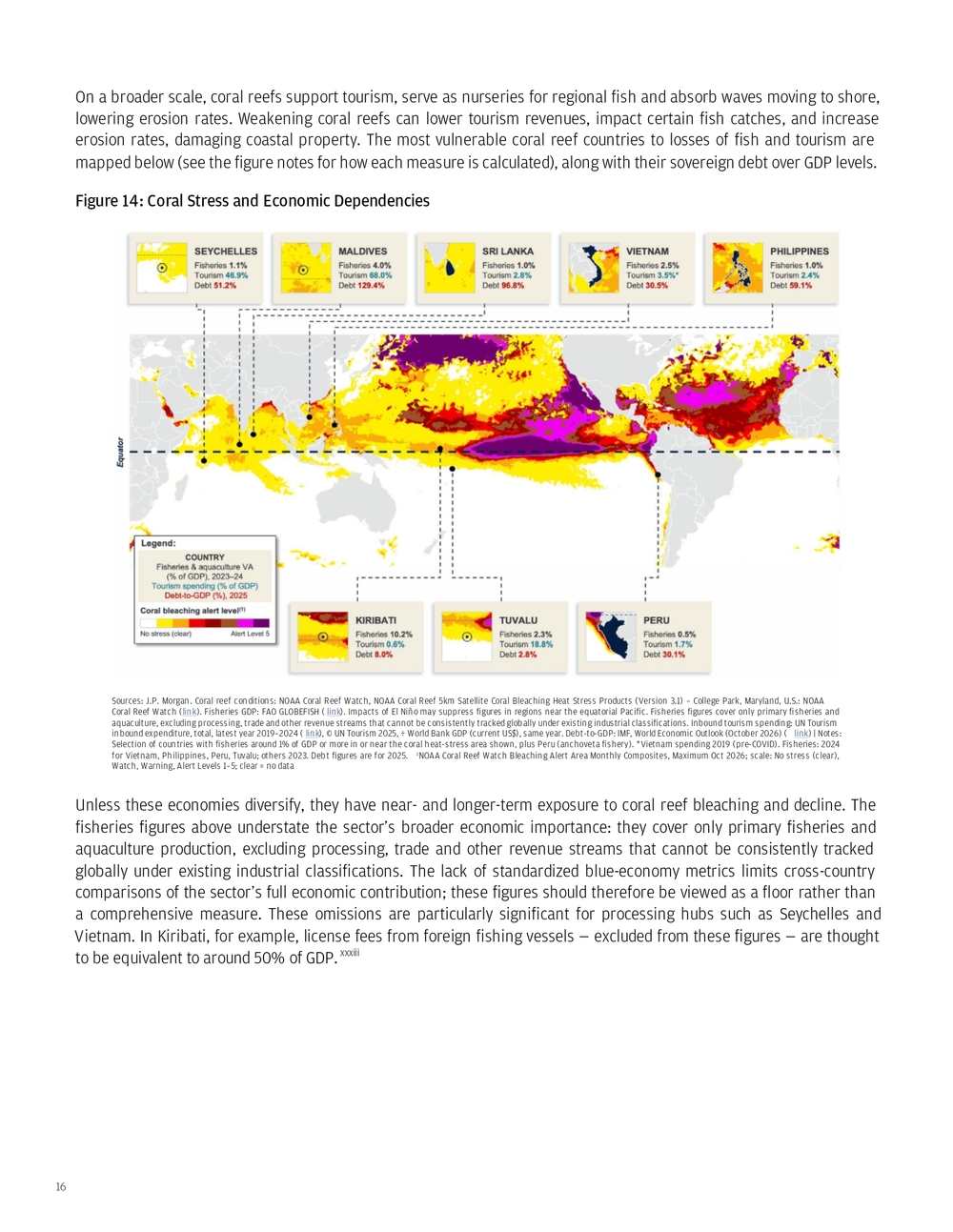
17 There are several places globally that are currently experiencing disruptions to business operations due to drought. They need water in their next wet season, or even simply the next few months — otherwise, the drought impact of recent months could extend. Should there be insufficient recovery in the cooler winter months in the Northern Hemisphere, the summer 2026 disruptions could return and be exacerbated by the predicted unprecedented summer heat of 2027 as the El Niño slowly dissipates. These impacts are not just in agriculture, but also extend to transportation, power generation and industry. What connects these regions is water’s role as critical infrastructure; instead of being treated as ephemeral, it may have been assumed to be available in its historic state over the long term. The immediate disruption may involve electricity generation, shipping capacity or municipal supplies, but the underlying challenge is the same: whether the next wet season provides enough replenishment to rebuild a buffer before the summer heat requires water for cooling or surface waters evaporate at greater speeds in a hotter world. A short-term improvement can ease operating constraints without resolving the longer-term surface shortage problem. 4. All eyes on water: The shortages are systemic and historic, but the El Niño heat won’t help in the coming year Figure 15: El Niño Rainfall Outlook (Nov–Jan) and Latest Monitoring Indicators Sources: WMO Global Seasonal Climate Update, Nov–Jan 2026/27 ( link); USDA PSD ( link); Ember ( link); Reclamation: Powell ( link), Mead ( link); USACE, Memphis ( link); WSV, Kaub ( link); USGS, Choke Canyon ( link); Corpus Christi (City) ( link); USDA AgTransport, St. Louis barge rates ( link); Bloomberg (Peru, Chile mining); World Bank; Panama Canal Authority | Notes: Crops: USDA 2026/27 vs 2025/26 forecasts (Nov., except Thai sugar Oct. and coffee July). Mining: single month vs a year earlier (Peru Aug., Chile Sep.). Barge rate: week of Oct. 27, YoY. Hydro output: Jun–Sep, YoY. Reservoirs: Nov. 1 vs a year earlier (Choke Canyon: vs 2000–25 same-date median). River gauges: Nov. 1 vs 2000–25 same-date median (Kaub daily means; Memphis 8 a.m.), relative to gauge zero
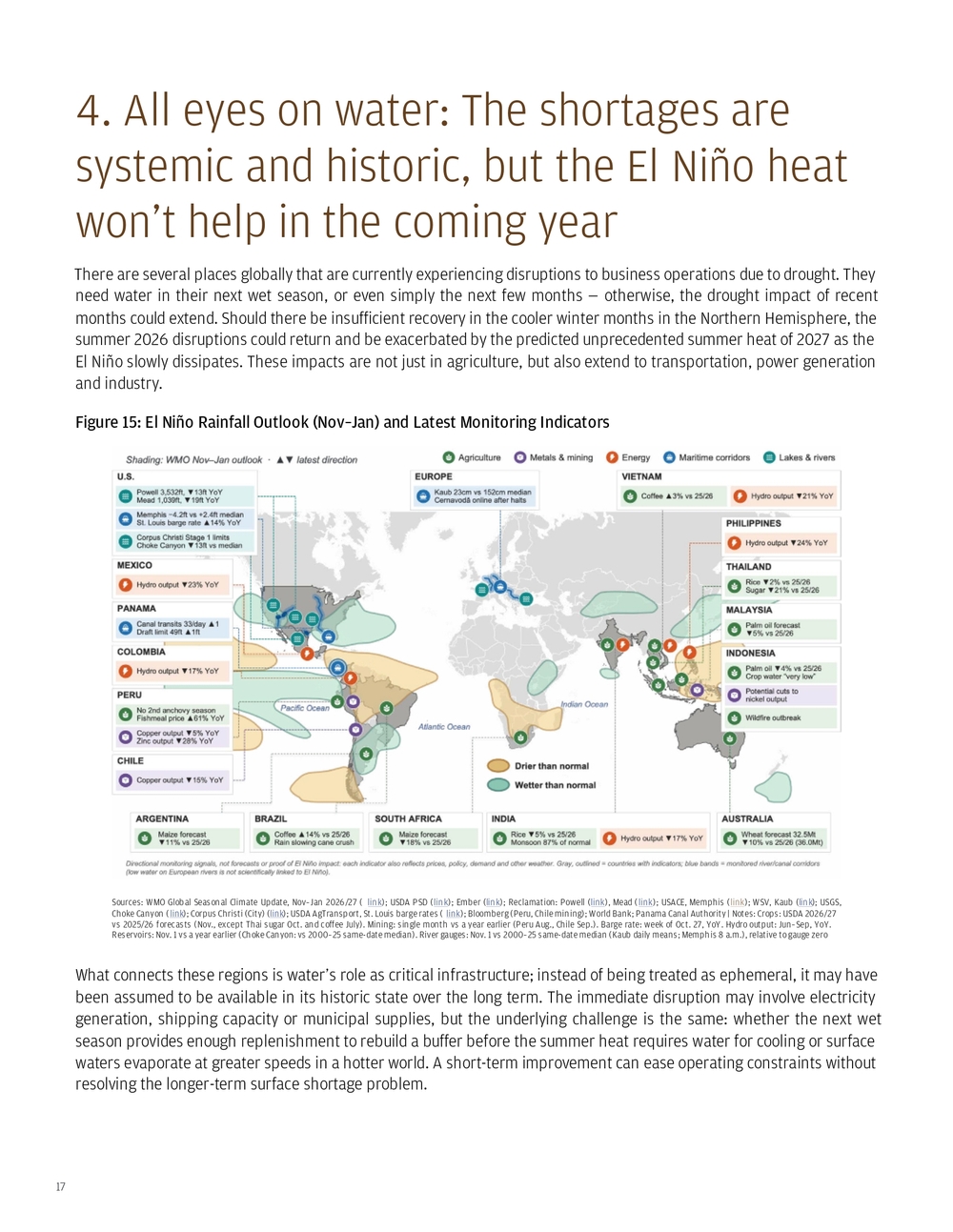
18 Energy generation is one area where those water shortages are already creating operational concerns via two pathways: Low Rhine levels are restricting coal deliveries to German power plants, with generation constraints reported through the end of November at Walsum 10 and through year-end at Mannheim. xxxiv The Kaub Rhine gauge has registered the lowest level since at least 2000 and is well below normal variability. On the Danube, Romania’s Cernavoda reactors depend on river water for cooling. Low Danube levels halted the plant from mid-August, and the operator tied restarts to water-level forecasts; both units were reconnected in November as river levels rose. xxxv Put another way, enough precipitation needs to fall—and remain in the forecast—for the nuclear operator to plan for months of sustained power production, rather than a short-lived restart followed by renewed water constraints. Even power plants with high self-sufficiency through minimal fuel transport xxxvi are exposed through their current cooling systems. In both locations, the forecast for the next few months is for average precipitation. Figure 16: Watching Water Sources: German Federal Waterways and Shipping Administration (WSV), PEGELONLINE, Kaub water level, daily means of 15-minute readings, Jan. 1, 2000–Nov. 1, 2026 ( link). Panama Canal Authority; public research | Notes: The band shows the 10th–90th percentile and the line the median of daily mean Kaub readings for each calendar day across 2000–2025; 2026 data through Nov. 1. The Kaub gauge is a reference reading, not the depth of the shipping channel; ships can still pass at low or negative readings with reduced loads The Panama Canal is part of a freshwater system, reliant on Gatun Lake to supply the locks and move vessels through the canal.xxxvii As water levels decline in drought, fewer container ships can traverse per day. Near-average rainfall in September and October, coupled with municipal water-saving measures, allowed the Canal Authority to increase daily transit slots to 33 on October 15.xxxviii That represents a partial easing of restrictions, but not the disappearance of water risk. The current outlook through January is for below-average precipitation in the region, and the Canal Authority has warned that shortages are expected to continue. Transportation managers need to carefully follow this guidance as vessels without advance reservations could face indefinite delays waiting for a transportation slot.xxxix While emergency freshwater saving measures are currently helping to avoid further restrictions, full relief is not expected through the main rainy season (which ends in December).
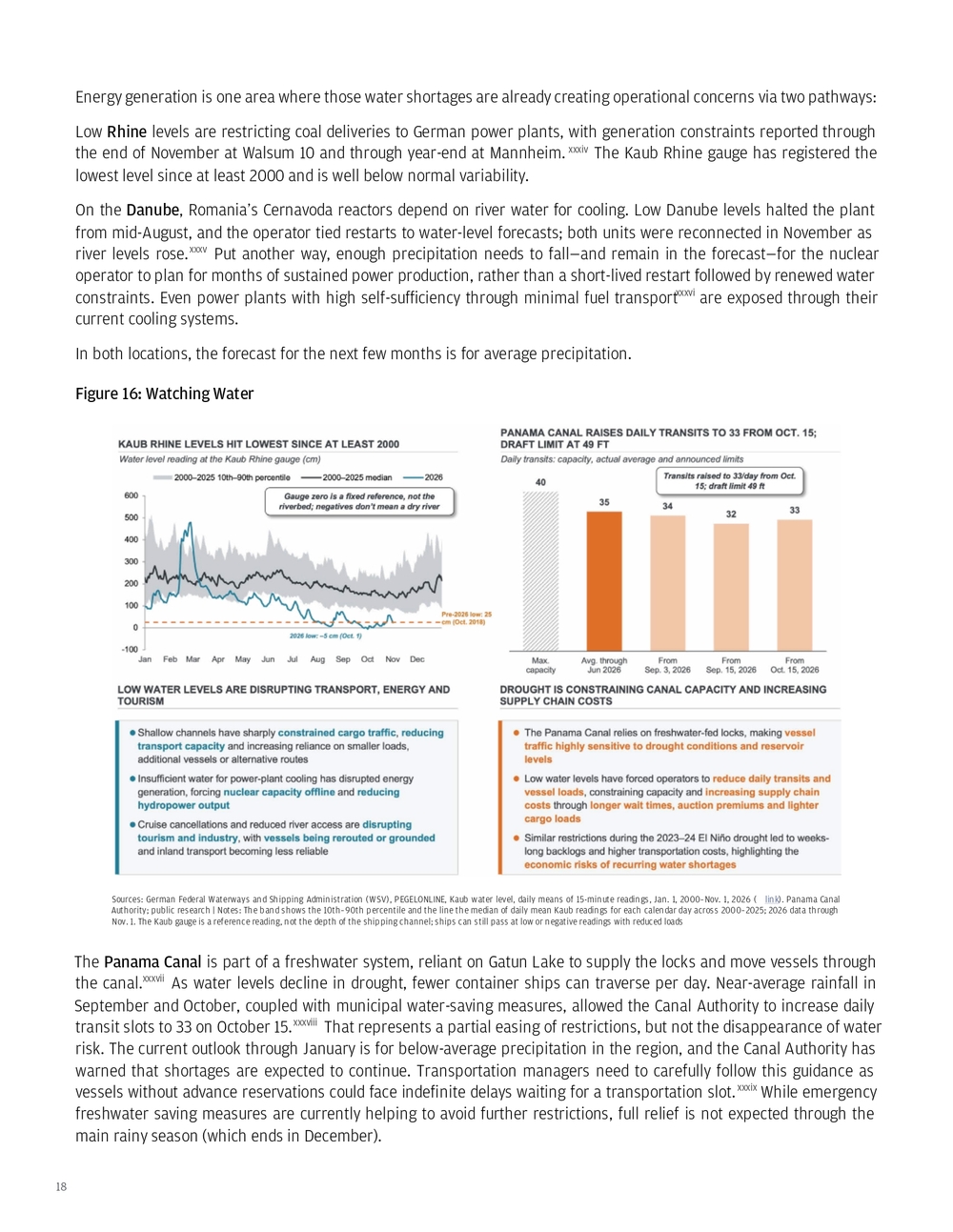
19 Corpus Christi, Texas has been under increasing water restrictions in recent months as surface supplies have declined across a multi-year drought. As of November 1, Lake Corpus Christi has recovered to near its 2000–2024 same-date median following exceptionally low spring levels, while Choke Canyon — the system’s largest reservoir — remained approximately 13 feet below its same-date median. Summer rainfall improved the supply outlook: reporting in August put the projected onset of a Level 1 water emergency in September 2028, although Stage 1 restrictions remained in place in early November.xl Recent rainfall has bought time to strengthen resilience in this region. Corpus Christi is a major energy-export hubxli, and the region’s refineries and chemical plants together use more water than its approximately 500,000 residents.xlii Figure 17: Corpus Christi Water Dashboard Sources: 1Lake levels: U.S. Geological Survey, daily lake elevation for Lake Corpus Christi ( link), Choke Canyon ( link) and Lake Texana ( link); 2Restrictions: City of Corpus Christi ( link); Drought Contingency Plan (stage triggers; Lake Texana excluded) ( link); Stage 1 site (link); Texas Tribune (outlook) ( link); Corpus Christi Caller-Times (Prop B) ( link); 3Industries: CNBC citing Port of Corpus Christi CEO (exports) ( link); Inside Climate News (industrial water use) ( link); Texas Real Estate Research Center (employers, services) ( link) | Notes: USGS daily maximum lake elevation (Lake Corpus Christi and Choke Canyon: NGVD 1929; Lake Texana: NAVD 1988); Median = calendar-day median, 2000–2024 (Texana 2007–2024) The Colorado River Basinxliii has also experienced a multi-year drought, leading to the decline of reservoir levels and water availability for multiple industries (farming, municipal governments, industry, hydropower production). The basin’s 2026 snow accumulation peaked well below its historical median. By November 1, Lake Powell’s elevation had recovered slightly to 3,532 feet but remained approximately 92 feet below its 1991–2020 median for that date. Lake Mead stood at 1,039 feet — approximately 88 feet below its same-date median and 19 feet below its level a year earlier.
20 Figure 18: Colorado River Dashboard Sources: 1Bureau of Reclamation, pool elevation: Powell ( link) / Mead (link); 2Drought.gov / USDA NRCS ( link); April 1 snow water equivalent as % of 1991–2020 median, western SNOTEL basins; 2026 data through March 30; 3USDA NRCS, Upper Colorado SNOTEL snow water equivalent; median 1991–2020 ( link) | Notes: 1Calendar-day median and 10th percentile, 1991–2020; daily data through Nov. 1, 2026 For the Colorado River, the key question is whether the winter wet season, from now through April/May, will build enough snowpack to sustain spring runoff and replenish reservoirs before summer. Warm to unclear (equal chance warm or cold) conditions with leaning-above or unclear (equal chance wet or dry) precipitation are expected in the upper basin, making reservoir recovery unlikely. Exceptionally wet years are increasingly needed to reduce deficits as warmer springs and summers increase evaporation before water reaches reservoirs (Milly and Dunne, Science, 2020).
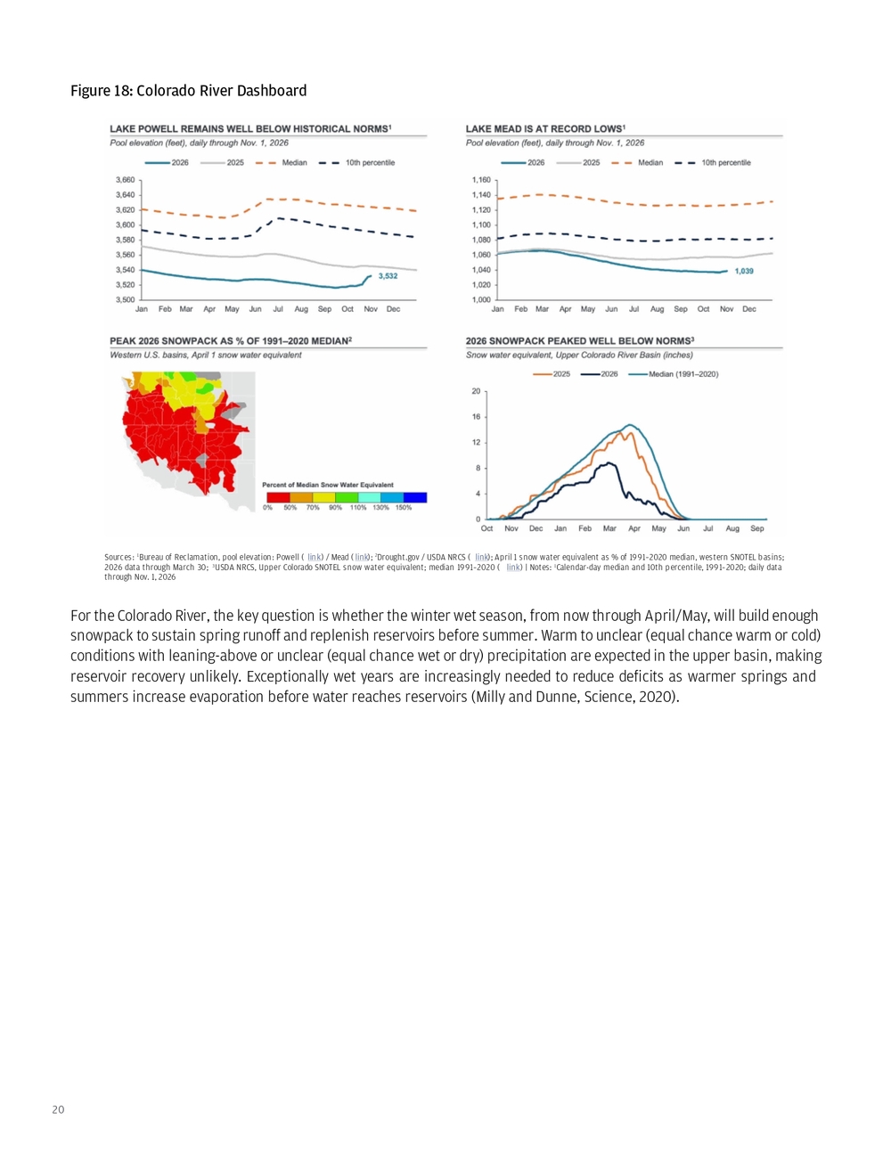
21 Figure 19: Seasonal Outlook: Dec-Feb Sources: NOAA Climate Prediction Center, official three-month temperature and precipitation outlooks for Dec–Jan–Feb 2026–27 (0.5-month lead), issued Nov. 19, 2026 ( link); NOAA Climate Prediction Center, prognostic discussion for long-lead seasonal outlooks ( link) | Notes: Normal is the 1991–2020 average; Equal Chances = odds similar to climatology River levels, reservoir storage and snowpack provide different pieces of the water picture. They should not all be interpreted as evidence of El Niño causation, particularly in Europe. Rather, they help identify systems entering the coming year with limited water buffers, where disappointing replenishment from precipitation in the coming months or exceptional 2027 heat (caused by climate change plus a temporary increase from El Niño) could prolong existing shortages. Increasingly, corporate assets are being mapped to forecasts to anticipate potential business disruptions and analyze public company exposure. For example, the chart below maps expected lower precipitation regions to assets in the Russell 1000. Several regions are expected to experience low precipitation levels, including western Canada, Panama and the Amazon. These locations are expected to face continued water stress that may affect regional transportation and operations. In Canada, Brazil and Indonesia, expected prolonged drought would increase the likelihood of summer wildfires.
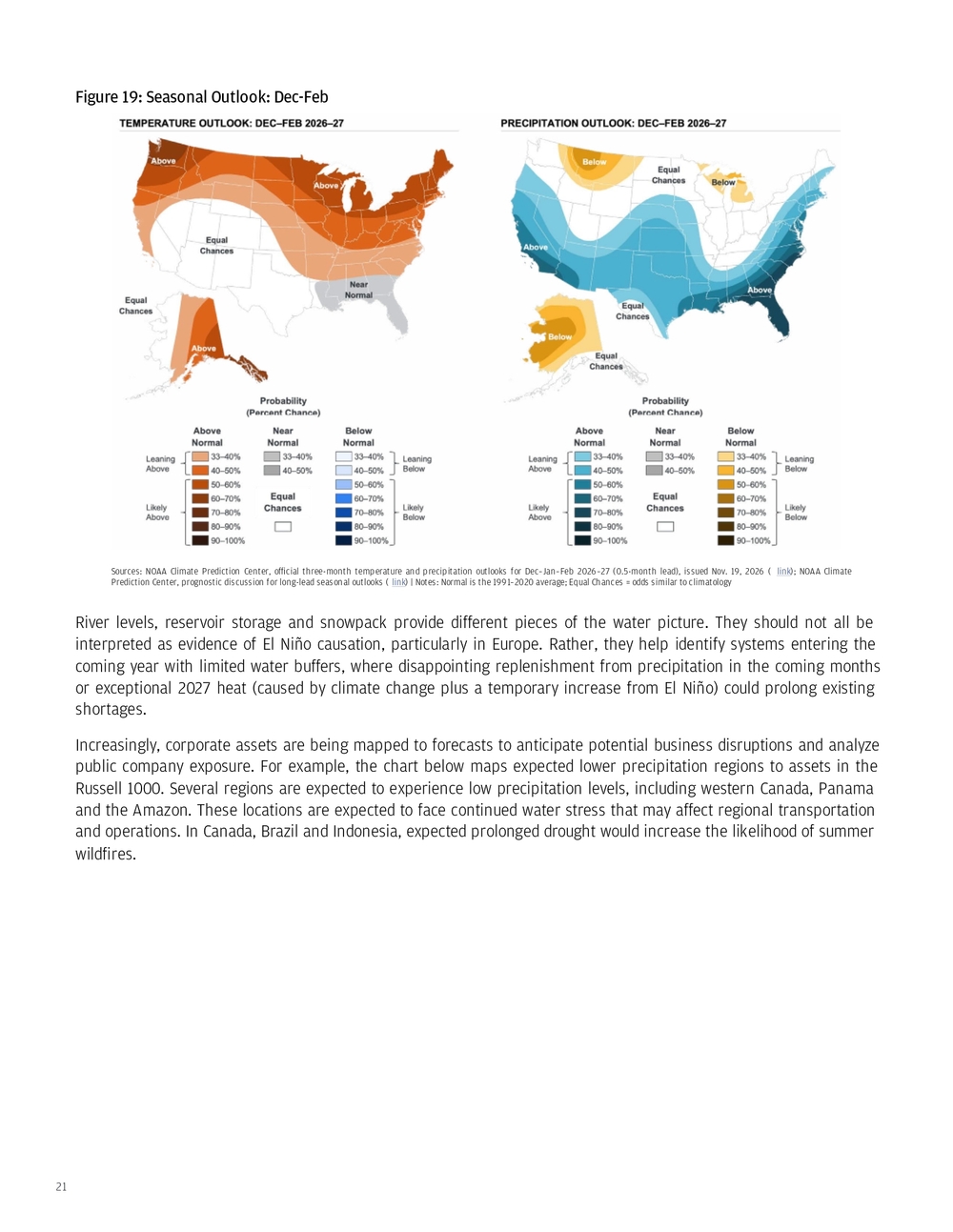
22 Figure 20: Share of Forecast Scenarios Indicating a Drier-Than-Normal Winter by Asset Location and Sector (%) Source: Kepler Labs | Notes: Data reflects the share of ECMWF SEAS5 51 forecast runs indicating December - February rainfall conditions drier than the 1991-2020 baseline. Colored shading indicates the percentage of forecast scenarios projecting a winter in the driest third of the 1991-2020 distribution. Asset markers are colored by sector, while marker size reflects annual revenue exposure within the affected region. Asset revenue is grouped into ranges, with circle size reflecting the corresponding revenue range. A normal winter corresponds to a value of 33%. The dark gray shaded areas see less than 5mm during this time of year, so they were left out of this analysis. Reproduced with permission for use in this paper only. The data and figure are provided as is and are based on the most recent cited forecast. They may not be reused or redistributed separately from this paper. The analysis and conclusions are those of JPMorganChase. This paper is not investment advice.
23 As the El Niño has developed into a strong event, I’ve been fielding questions from clients about how to interpret its impacts. Common questions include: • How should businesses and global leaders interpret short-term temperature spikes associated with El Niño against the longer-term warming averages and indexes used to assess climate goals? • If global temperatures exceed 1.5°C or approach 2°C (values set due to the Paris Agreement) for a month or a year, does that constitute a lasting breach, or might temperatures later return closer to prior levels? • For those whose decisions are aligned to these thresholds, what should an El Niño-related overshoot mean for their goals and choices? In February 2025, I explained the many definitions of how the 1.5°C or 2.0°C thresholds were calculated by scientists, and the spirit of how they were intended to be calculated for the Paris Agreement (a 30-year climatological average).xliv In 2024, major media releases highlighted crossing the threshold of 1.5°C for individual months; this threshold was also crossed for multiple data sets for all of 2024.xlv We’re about to come close to (if not cross) 2°C for an individual month, and will likely stay well above 1.5°C for the first half of 2027, and likely the full year. This potentially poses an issue for people who have made temperature-alignment decisions. Crossing 1.5°C for individual months — and approaching 2°C — can create a sense of urgency for those who have made decisions tied to staying below these thresholds. The UN Environment Programme now says some overshoots of 1.5°C are unavoidable. Its lowest- overshoot scenario peaks at 1.7–1.8°C around mid-century, even with deep emissions cuts and carbon removal. xlvi The globe could exceed 1.8°C in individual months this winter, although that is different from reaching that warming level over the long term. Definitions matter, yet they’ve often been ill-defined. At the precipice of thresholds being breached, critical questions for people making temperature-related decisions may now include: • If you align decisions to temperature outcomes, what does it mean when you exceed your threshold in a single year? • Are you waiting for specific data or thresholds to be crossed?xlvii A 30-year running average of temperature (climatological average used by scientists) or more recent history (reflecting more recent impacts and experience)? • At what point do you declare that the temperature threshold you set previously is dead and create a new goal? • Do you double down on emissions reduction technologies, with an additional focus on technologies that account for temperature overshoots above 1.5°C and attempt to bring them back to your goal? Put another way, do you then invest in climate intervention technologies with carbon removal and solar radiation modification to draw down excess greenhouse gases in the atmosphere and cool the planet? As I wrote in the spring, xlviii increased funding is going into early-stage technologies for climate intervention. This may be a signal that governments, xlix philanthropists and investors are betting these technologies may be needed if global temperatures are to remain below 1.5°C to 2.0°C. A recent academic-led assessment estimates annual carbon removal is currently at ~2 GtCO2 a year, compared with the ~9 GtCO2 needed per year by 2050 to limit warming to 1.5°C, alongside highly ambitious emissions reductions.l 5. Potential renewed conversations about temperature-alignment goals (for those who participate) after surpassing a threshold
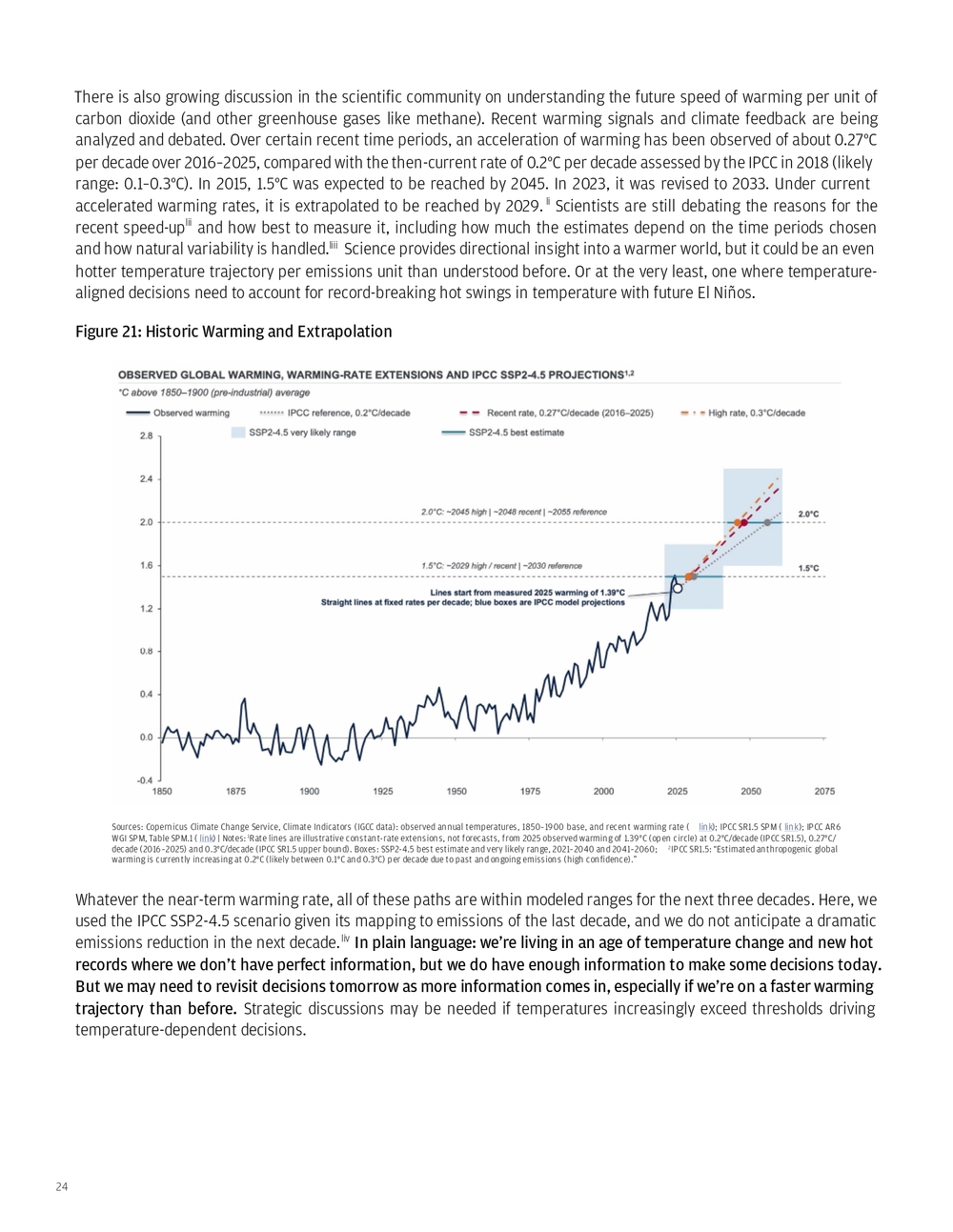
24 There is also growing discussion in the scientific community on understanding the future speed of warming per unit of carbon dioxide (and other greenhouse gases like methane). Recent warming signals and climate feedback are being analyzed and debated. Over certain recent time periods, an acceleration of warming has been observed of about 0.27°C per decade over 2016–2025, compared with the then-current rate of 0.2°C per decade assessed by the IPCC in 2018 (likely range: 0.1–0.3°C). In 2015, 1.5°C was expected to be reached by 2045. In 2023, it was revised to 2033. Under current accelerated warming rates, it is extrapolated to be reached by 2029. li Scientists are still debating the reasons for the recent speed-uplii and how best to measure it, including how much the estimates depend on the time periods chosen and how natural variability is handled.liii Science provides directional insight into a warmer world, but it could be an even hotter temperature trajectory per emissions unit than understood before. Or at the very least, one where temperature- aligned decisions need to account for record-breaking hot swings in temperature with future El Niños. Figure 21: Historic Warming and Extrapolation Sources: Copernicus Climate Change Service, Climate Indicators (IGCC data): observed annual temperatures, 1850–1900 base, and recent warming rate ( link); IPCC SR1.5 SPM ( link); IPCC AR6 WGI SPM, Table SPM.1 ( link) | Notes: 1Rate lines are illustrative constant-rate extensions, not forecasts, from 2025 observed warming of 1.39°C (open circle) at 0.2°C/decade (IPCC SR1.5), 0.27°C/ decade (2016–2025) and 0.3°C/decade (IPCC SR1.5 upper bound). Boxes: SSP2-4.5 best estimate and very likely range, 2021–2040 and 2041–2060; 2IPCC SR1.5: “Estimated anthropogenic global warming is currently increasing at 0.2°C (likely between 0.1°C and 0.3°C) per decade due to past and ongoing emissions (high confidence).” Whatever the near-term warming rate, all of these paths are within modeled ranges for the next three decades. Here, we used the IPCC SSP2-4.5 scenario given its mapping to emissions of the last decade, and we do not anticipate a dramatic emissions reduction in the next decade.liv In plain language: we’re living in an age of temperature change and new hot records where we don’t have perfect information, but we do have enough information to make some decisions today. But we may need to revisit decisions tomorrow as more information comes in, especially if we’re on a faster warming trajectory than before. Strategic discussions may be needed if temperatures increasingly exceed thresholds driving temperature-dependent decisions.
25 Dr. Sarah Kapnick Managing Director, Global head of Climate Advisory, Commercial & Investment Bank J.P. Morgan Climate Advisory Bringing science, technology, and policy expertise to market Climate Advisory works to help clients achieve their long- term strategic goals by providing in-depth insights at the intersection of science and finance With scientific expertise, we help clients navigate climate, energy, biodiversity and sustainability topics so they can adapt to challenges and realize the opportunities ahead • Helping clients navigate climate challenges with insights and scientific research • Delivering thought leadership on climate-related strategies across finance, science, technology, physical risk, national security and geopolitics Combining scientific, fact-based assessments and practical application, the Climate Intuition series highlights the impacts of climate change on strategic decision-making Climate Intuition Series All Climate Intuition publications A guide to enabling resilience discussions Balancing the energy security equation Food security under pressure: Iran conflict and a brewing El Niño Sign up to receive in your inbox Recent publications All Climate Advisory content can be found at https:/ /www.jpmorgan.com/investment-banking/climate-advisory CLIENT ADVISORY LEADERSHIP AND INSIGHTS CLIENT INTUITION SERIES
26 FOOTNOTES i. https://www.ncei.noaa.gov/news/global-climate-202513 ii. Assuming a current warming path of 0.2–0.3°C. per decade or following along an emissions path of SSP2-4.5. iii. https://www.jpmorgan.com/insights/sustainability/climate/food-security-under-pressure iv. Lemoine, D., Kapnick, S. Financial markets value skillful forecasts of seasonal climate. Nat Commun 15, 4059 (2024). https://doi.org/10.1038/s41467- 024-48420-z v. Bloomberg, end-of-day futures prices on June 11, 2026 (the day El Niño was declared) and Nov. 2, 2026. Each change compares the March 2027 contract on both dates: ICE cocoa, ICE arabica coffee, ICE sugar #11, and CBOT rough rice, corn and wheat. vi. https://www.foreignaffairs.com/united-states/avoiding-next-famine vii. European Central Bank, Risks to global food commodity prices from El Niño ( link) viii. European Central Bank, Has food inflation lost its bite? ( link) ix. USDA Foreign Agricultural Service, Production, Supply and Distribution (PSD) database, downloaded Nov. 10, 2026 (November WASDE update) x. https://www.jpmorgan.com/insights/sustainability/climate/food-security-under-pressure xi. https://www.cfr.org/articles/hunger-on-the-horizon-the-new-black-sea-grain-crisis xii. FAOSTAT, Crops and livestock products, production quantity, 2024 xiii. Drewry World Container Index, via Bloomberg; $1,898.54 per 40-foot container on Feb. 26, 2026 (pre-conflict), versus $4,389.04 on Nov. 5, 2026—an increase of 131.2% https://www.drewry.co.uk/supply-chain-advisors/supply-chain-expertise/world-container-index-assessed-by-drewry xiv. https://www.fas.usda.gov/newsroom/usda-invests-825-million-america-first-international-food-assistance , https://www.fas.usda.gov/newsroom/ usda-purchase-211000-metric-tons-american-commodities-administer-food-peace-program xv. https://www.globalhungerindex.org/perspectives/regional-perspectives/horn-of-africa.html xvi. https://www.fas.usda.gov/data/gain-report/2026/02/Drought%20Dampens%20Crop%20Production%20in%20Central%20Kenya_Nairobi_Kenya_ KE2026-0003.pdf ; https://www.fao.org/giews/countrybrief/country.jsp?code=KEN and https://www.unocha.org/news/acting-early-ethiopia-when- world-isnt-watching xvii. https://pubs.usgs.gov/periodicals/mcs2026/mcs2026-cobalt.pdf xviii. https://www.ifpri.org/blog/how-are-fertilizer-markets-coping-with-the-continued-closure-of-the-strait-of-hormuz/ xix. https://www.climate.gov/news-features/understanding-climate/climate-change-ocean-heat-content xx. History lesson: old ship tracks were used to identify the first “zones” to define El Niño. Eventually, zones 3 and 4 were merged into “3.4” as research studies showed the region was more useful for identifying further El Niño development and associated impacts on land. xxi. This ensemble is made up of several models from different centers across the U.S. and Canada to generate a 12-month seasonal forecast. xxii. https://wmo.int/news/media-centre/new-report-suggests-more-global-temperature-records-ahead xxiii. https://www.euronews.com/2026/10/08/eu-faces-gas-shortfall-of-up-to-15-if-severe-winter-hits-report-warns and https://www.entsog.eu/ xxiv. Scaife, A. A., Baldwin, M. P., Butler, A. H., Charlton-Perez, A. J., Domeisen, D. I. V., Garfinkel, C. I., Hardiman, S. C., Haynes, P., Karpechko, A. Y., Lim, E.-P., Noguchi, S., Perlwitz, J., Polvani, L., Richter, J. H., Scinocca, J., Sigmond, M., Shepherd, T. G., Son, S.-W., and Thompson, D. W. J.: Long-range prediction and the stratosphere, Atmos. Chem. Phys., 22, 2601–2623, https://doi.org/10.5194/acp-22-2601-2022, . An SSW developed in November 2026. It was well forecasted 2 weeks in advance and as of writing, is dissipating. It is not expected to have a long term impact on SSW probability for the winter of 2026-27 as polar temperatures still have time to cool during SSW probability peak in January/February. This is a record-early event. For further SSW predictability reading: https://agupubs.onlinelibrary.wiley.com/doi/10.1029/2019JD030920 xxv. The famous weather forecasting Pennsylvania groundhog that sees its shadow or not to signify 6 more weeks of winter or early spring. xxvi. University of Miami Cooperative Institute for Marine & Atmospheric Studies and NOAA, Global Surface Temperature ( link) xxvii. This presumes emissions will not go net negative through carbon removal. Or that solar radiation modification is not deployed to globally cool the planet. Or a set of improbable science and geopolitical fiction scenarios that aren’t entirely impossible. xxviii. https://research.noaa.gov/50-years-of-getting-enso-predictions-mostly-correct/ xxix. https://globalocean.noaa.gov/research/argo-program/ xxx. https://www.bloomberg.com/news/articles/2026-07-15/peru-economy-misses-expectations-on-weak-fishing-and-manufacture xxxi. https://www.bloomberg.com/news/articles/2026-07-15/peru-economy-misses-expectations-on-weak-fishing-and-manufacture xxxii. Coral bleaching happens when corals get stressed (most often because the water gets too warm) and they push out the tiny algae that normally live inside them. This usually occurs when the water temperature rises to about 1°C (1.8°F) above the highest temperature that’s normal for that area. If water temperatures stay hot for too long, the algae don’t return and coral tissues die. https://oceanservice.noaa.gov/facts/coral_bleach.html xxxiii. FAO, Fisheries and Aquaculture Division
27 FOOTNOTES xxxiv. https://www.bloomberg.com/news/articles/2026-10-09/low-rhine-curbs-coal-supplies-at-steag-german-power-plant xxxv. https://www.world-nuclear-news.org/articles/cernavoda-units-remain-offline-due-to-danube-water-levels , https://serbia-energy.eu/romania- begins-restarting-cernavoda-nuclear-generation-after-danube-drought/ xxxvi. See Figure 61 of https://jpmorgan.celero.site/s/26e72c0b/jpmc-cfg-energy-sept-2026-v6/?page=1 xxxvii. https://pancanal.com/en/first-panama-canal-water-saving-basin-filled-testing-process-begins/ xxxviii. https://pancanal.com/en/panama-canal-announces-increase-in-draft-and-daily-transit/ xxxix. Advisory to Shipping No. A-36-2026: https://pancanal.com/wp-content/uploads/2026/04/ADV-36-2026-Increase-in-the-Number-of-Neopanamax- Booking-Slots-Draft-Adjustment-and-Transit-Reservation-System.pdf xl. https://stage1.corpuschristitx.gov/ xli. https://www.cnbc.com/2026/05/03/us-crude-oil-exports-surge-to-record-as-tankers-flock-to-gulf-coast.html xlii. https://www.yahoo.com/news/us/articles/corpus-christi-texas-bet-desalination-074700566.html xliii. Upper basin states: Colorado, New Mexico, Utah, and Wyoming. Lower basin states: Arizona, California, and Nevada. xliv. https://www.jpmorgan.com/insights/sustainability/climate/navigating-the-new-climate-era xlv. https://climate.copernicus.eu/copernicus-2024-first-year-exceed-15degc-above-pre-industrial-level xlvi. UN Environment Programme, Emissions Gap Report 2026 ( link) xlvii. Table 1 in: https://www.jpmorgan.com/content/dam/jpm/cib/documents/Building_intuition_for_strategic_decision_making.pdf xlviii. https://jpmorgan.celero.site/s/ab29c67c/climate-intuition-tipping-points/?page=1 xlix. https://www.nature.com/articles/d41586-026-03415-2 l. Carbon dioxide removal totals 2.2 GtCO 2 per year, equivalent to 5% of gross CO 2 emissions, but is overwhelmingly conventional (afforestation, reforestation, wood products). To be specific, 99.9% comes from conventional CDR, concentrated in China, the United States, the European Union, Brazil, and Russia. From: The State of Carbon Dioxide Removal, 3rd edition (2026), Chapter 7, “Current levels of CDR,” and Chapter 9, “The CDR gap,” p. 224. Figures rounded from 2.2 and 8.8 GtCO 2 per year, respectively ( link) li. https://climate.copernicus.eu/how-fast-world-has-moved-closer-15degc-global-warming-paris-agreement lii. There are several hypotheses for accelerating warming today, including: natural variability (brief fast warming which will normalize back to previous levels) and reduced air pollution that reflected sunlight (sulfur dioxide from ships). liii. https://indicators.climate.copernicus.eu/ and https://www.ipcc.ch/sr15/chapter/spm/ liv. https://www.jpmorgan.com/insights/sustainability/climate/navigating-the-new-climate-era